How To Draw 0db Per Dec In Matlab

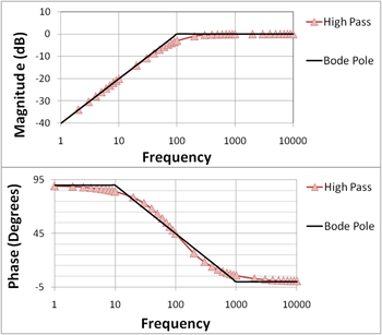
Effigy 1A: The Bode plot for a first-club (ane-pole) highpass filter; the straight-line approximations are labeled "Bode pole"; stage varies from ninety° at low frequencies (due to the contribution of the numerator, which is 90° at all frequencies) to 0° at high frequencies (where the stage contribution of the denominator is −90° and cancels the contribution of the numerator).

Effigy 1B: The Bode plot for a first-gild (one-pole) lowpass filter; the straight-line approximations are labeled "Bode pole"; phase is 90° lower than for Effigy 1A because the phase contribution of the numerator is 0° at all frequencies.

In electrical engineering science and control theory, a Bode plot is a graph of the frequency response of a arrangement. It is ordinarily a combination of a Bode magnitude plot, expressing the magnitude (usually in decibels) of the frequency response, and a Bode phase plot, expressing the phase shift.

As originally conceived by Hendrik Wade Bode in the 1930s, the plot is an asymptotic approximation of the frequency response, using straight line segments.^[ane]

Overview [edit]

Among his several of import contributions to circuit theory and control theory, engineer Hendrik Wade Bode, while working at Bong Labs in the 1930s, devised a unproblematic simply authentic method for graphing proceeds and phase-shift plots. These acquit his proper name, Bode gain plot and Bode phase plot. "Bode" is often pronounced BOH-dee although the Dutch pronunciation is Bo-duh. (Dutch: [ˈboːdə]).^{[2] [iii]}

Bode was faced with the problem of designing stable amplifiers with feedback for utilize in telephone networks. He developed the graphical design technique of the Bode plots to show the gain margin and phase margin required to maintain stability under variations in circuit characteristics acquired during manufacture or during operation.^[4] The principles developed were applied to blueprint issues of servomechanisms and other feedback control systems. The Bode plot is an case of assay in the frequency domain.

Definition [edit]

The Bode plot for a linear, fourth dimension-invariant system with transfer function ${\displaystyle H(s)}$ ( ${\displaystyle s}$ existence the complex frequency in the Laplace domain) consists of a magnitude plot and a phase plot.

The Bode magnitude plot is the graph of the function ${\displaystyle |H(s=j\omega )|}$ of frequency ${\displaystyle \omega }$ (with ${\displaystyle j}$ existence the imaginary unit). The ${\displaystyle \omega }$ -axis of the magnitude plot is logarithmic and the magnitude is given in decibels, i.e., a value for the magnitude ${\displaystyle |H|}$ is plotted on the centrality at ${\displaystyle 20\log _{ten}|H|}$ .

The Bode stage plot is the graph of the phase, commonly expressed in degrees, of the transfer function ${\displaystyle \arg \left(H(s=j\omega )\right)}$ as a function of ${\displaystyle \omega }$ . The phase is plotted on the same logarithmic ${\displaystyle \omega }$ -axis equally the magnitude plot, but the value for the phase is plotted on a linear vertical axis.

Frequency response [edit]

This department illustrates that a Bode Plot is a visualization of the frequency response of a system.

Consider a linear, time-invariant system with transfer function ${\displaystyle H(due south)}$ . Assume that the system is subject to a sinusoidal input with frequency ${\displaystyle \omega }$ ,

${\displaystyle u(t)=\sin(\omega t)\;,}$

that is practical persistently, i.e. from a fourth dimension ${\displaystyle -\infty }$ to a time ${\displaystyle t}$ . The response volition exist of the form

${\displaystyle y(t)=y_{0}\sin(\omega t+\varphi )\;,}$

i.due east., also a sinusoidal signal with aamplitude ${\displaystyle y_{0}}$ shifted in phase with respect to the input by a phase ${\displaystyle \varphi }$ .

It can be shown^[v] that the magnitude of the response is

${\displaystyle y_{0}=|H(\mathrm {j} \omega )|}$

(1)

and that the phase shift is

${\displaystyle \varphi =\arg H(\mathrm {j} \omega )\;.}$

(2)

A sketch for the proof of these equations is given in the appendix.

In summary, subjected to an input with frequency ${\displaystyle \omega }$ the organisation responds at the aforementioned frequency with an output that is amplified by a factor ${\displaystyle |H(\mathrm {j} \omega )|}$ and phase-shifted by ${\displaystyle \arg(H(\mathrm {j} \omega ))}$ . These quantities, thus, characterize the frequency response and are shown in the Bode plot.

Rules for handmade Bode plot [edit]

For many practical issues, the detailed Bode plots can be approximated with straight-line segments that are asymptotes of the precise response. The effect of each of the terms of a multiple element transfer role can exist approximated by a set of straight lines on a Bode plot. This allows a graphical solution of the overall frequency response office. Before widespread availability of digital computers, graphical methods were extensively used to reduce the need for boring calculation; a graphical solution could be used to place viable ranges of parameters for a new blueprint.

The premise of a Bode plot is that one tin can consider the log of a function in the form:

${\displaystyle f(x)=A\prod (x-c_{n})^{a_{n}}}$

as a sum of the logs of its zeros and poles:

${\displaystyle \log(f(10))=\log(A)+\sum a_{n}\log(x-c_{n})\;.}$

This idea is used explicitly in the method for cartoon stage diagrams. The method for cartoon amplitude plots implicitly uses this idea, just since the log of the amplitude of each pole or null always starts at zilch and only has one asymptote change (the directly lines), the method can be simplified.

Straight-line amplitude plot [edit]

Amplitude decibels is unremarkably washed using ${\displaystyle {\text{dB}}=20\log _{10}(10)}$ to define decibels. Given a transfer role in the form

${\displaystyle H(south)=A\prod {\frac {(s-x_{northward})^{a_{n}}}{(s-y_{n})^{b_{due north}}}}}$

where ${\displaystyle x_{due north}}$ and ${\displaystyle y_{n}}$ are constants, ${\displaystyle s=\mathrm {j} \omega }$ , ${\displaystyle a_{n},b_{n}>0}$ , and ${\displaystyle H}$ is the transfer function:

To handle irreducible second society polynomials, ${\displaystyle ax^{2}+bx+c}$ can, in many cases, be approximated as ${\displaystyle ({\sqrt {a}}ten+{\sqrt {c}})^{two}}$ .

Annotation that zeros and poles happen when ${\displaystyle \omega }$ is equal to a sure ${\displaystyle x_{northward}}$ or ${\displaystyle y_{northward}}$ . This is considering the function in question is the magnitude of ${\displaystyle H(\mathrm {j} \omega )}$ , and since it is a complex function, ${\displaystyle |H(\mathrm {j} \omega )|={\sqrt {H\cdot H^{*}}}}$ . Thus at any place where there is a zero or pole involving the term ${\displaystyle (s+x_{n})}$ , the magnitude of that term is ${\textstyle {\sqrt {(x_{n}+\mathrm {j} \omega )\cdot (x_{n}-\mathrm {j} \omega )}}={\sqrt {x_{n}^{2}+\omega ^{2}}}}$ .

Corrected aamplitude plot [edit]

To right a straight-line amplitude plot:

Annotation that this correction method does non incorporate how to handle complex values of ${\displaystyle x_{n}}$ or ${\displaystyle y_{n}}$ . In the instance of an irreducible polynomial, the best way to correct the plot is to really calculate the magnitude of the transfer function at the pole or naught corresponding to the irreducible polynomial, and put that dot over or under the line at that pole or zilch.

Straight-line phase plot [edit]

Given a transfer part in the aforementioned form as above:

${\displaystyle H(s)=A\prod {\frac {(s-x_{n})^{a_{n}}}{(s-y_{n})^{b_{n}}}}}$

the thought is to draw separate plots for each pole and zero, then add them up. The actual stage curve is given by ${\displaystyle -\arctan \left({\tfrac {\mathrm {Im} [H(south)]}{\mathrm {Re} [H(s)]}}\correct)}$ .

To draw the phase plot, for each pole and null:

• If ${\displaystyle A}$ is positive, start line (with zero slope) at ${\displaystyle 0^{\circ }}$
• If ${\displaystyle A}$ is negative, get-go line (with zip gradient) at ${\displaystyle -180^{\circ }}$
• If the sum of the number of unstable zeros and poles is odd, add 180° to that basis
• At every ${\displaystyle \omega =|x_{n}|}$ (for stable zeros ${\displaystyle -\operatorname {Re} (z)<0}$ ), increment the slope by ${\displaystyle 45\cdot a_{due north}}$ degrees per decade, showtime i decade before ${\displaystyle \omega =|x_{north}|}$ (East.m.: ${\textstyle {\frac {|x_{n}|}{10}}}$ )
• At every ${\displaystyle \omega =|y_{n}|}$ (for stable poles ${\displaystyle -\operatorname {Re} (p)<0}$ ), decrease the slope by ${\displaystyle 45\cdot b_{n}}$ degrees per decade, first one decade before ${\displaystyle \omega =|y_{northward}|}$ (E.yard.: ${\textstyle {\frac {|y_{n}|}{x}}}$ )
• "Unstable" (right half aeroplane) poles and zeros ( ${\displaystyle \operatorname {Re} (s)>0}$ ) take opposite behavior
• Flatten the gradient again when the phase has changed by ${\displaystyle 90\cdot a_{n}}$ degrees (for a zero) or ${\displaystyle xc\cdot b_{n}}$ degrees (for a pole),
• Later plotting 1 line for each pole or nil, add the lines together to obtain the final phase plot; that is, the terminal phase plot is the superposition of each before phase plot.

Example [edit]

To create a straight-line plot for a commencement-club (one-pole) lowpass filter, one considers the transfer function in terms of the angular frequency:

${\displaystyle H_{\mathrm {lp} }(\mathrm {j} \omega )={ane \over 1+\mathrm {j} {\omega \over {\omega _{\mathrm {c} }}}}\;.}$

The in a higher place equation is the normalized form of the transfer function. The Bode plot is shown in Figure ane(b) above, and structure of the direct-line approximation is discussed adjacent.

Magnitude plot [edit]

The magnitude (in decibels) of the transfer function higher up, (normalized and converted to angular frequency form), given by the decibel gain expression ${\displaystyle A_{\mathrm {vdB} }}$ :

${\displaystyle {\begin{aligned}A_{\mathrm {vdB} }&=20\cdot \log |H_{\mathrm {lp} }(\mathrm {j} \omega )|\\&=20\cdot \log {\frac {i}{\left|ane+\mathrm {j} {\frac {\omega }{\omega _{\mathrm {c} }}}\right|}}\\&=-20\cdot \log \left|1+\mathrm {j} {\frac {\omega }{\omega _{\mathrm {c} }}}\right|\\&=-10\cdot \log \left(1+{\frac {\omega ^{2}}{\omega _{\mathrm {c} }^{two}}}\correct)\finish{aligned}}}$

And then plotted versus input frequency ${\displaystyle \omega }$ on a logarithmic scale, can be approximated past two lines and it forms the asymptotic (gauge) magnitude Bode plot of the transfer function:

These two lines meet at the corner frequency. From the plot, it can be seen that for frequencies well below the corner frequency, the excursion has an attenuation of 0 dB, respective to a unity pass band gain, i.e. the amplitude of the filter output equals the amplitude of the input. Frequencies in a higher place the corner frequency are attenuated – the higher the frequency, the higher the attenuation.

Stage plot [edit]

The phase Bode plot is obtained by plotting the phase angle of the transfer function given past

${\displaystyle \arg H_{\mathrm {lp} }(\mathrm {j} \omega )=-\tan ^{-1}{\omega \over {\omega _{\mathrm {c} }}}}$

versus ${\displaystyle \omega }$ , where ${\displaystyle \omega }$ and ${\displaystyle \omega _{\mathrm {c} }}$ are the input and cutoff angular frequencies respectively. For input frequencies much lower than corner, the ratio ${\displaystyle {\omega \over {\omega _{\mathrm {c} }}}}$ is pocket-sized and therefore the phase angle is close to zero. As the ratio increases the absolute value of the phase increases and becomes −45 degrees when ${\displaystyle \omega =\omega _{\mathrm {c} }}$ . Equally the ratio increases for input frequencies much greater than the corner frequency, the phase bending asymptotically approaches −90 degrees. The frequency scale for the phase plot is logarithmic.

Normalized plot [edit]

The horizontal frequency centrality, in both the magnitude and phase plots, can be replaced by the normalized (nondimensional) frequency ratio ${\displaystyle {\omega \over {\omega _{\mathrm {c} }}}}$ . In such a case the plot is said to be normalized and units of the frequencies are no longer used since all input frequencies are at present expressed as multiples of the cutoff frequency ${\displaystyle \omega _{\mathrm {c} }}$ .

An instance with naught and pole [edit]

Figures two-five further illustrate construction of Bode plots. This instance with both a pole and a cypher shows how to apply superposition. To begin, the components are presented separately.

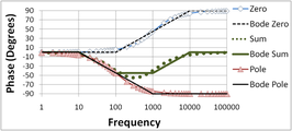
Figure 2 shows the Bode magnitude plot for a zero and a low-laissez passer pole, and compares the two with the Bode straight line plots. The directly-line plots are horizontal up to the pole (zero) location and so drop (rise) at 20 dB/decade. The second Figure three does the same for the phase. The stage plots are horizontal up to a frequency factor of ten below the pole (naught) location and so drop (rise) at 45°/decade until the frequency is ten times higher than the pole (zero) location. The plots then are again horizontal at higher frequencies at a final, full phase change of 90°.

Figure 4 and Figure v prove how superposition (simple addition) of a pole and zero plot is done. The Bode straight line plots once again are compared with the exact plots. The zilch has been moved to higher frequency than the pole to make a more interesting example. Notice in Figure 4 that the 20 dB/decade drop of the pole is arrested by the 20 dB/decade rise of the zero resulting in a horizontal magnitude plot for frequencies above the zero location. Discover in Figure 5 in the phase plot that the direct-line approximation is pretty approximate in the region where both pole and zero affect the phase. Detect also in Figure 5 that the range of frequencies where the phase changes in the direct line plot is limited to frequencies a factor of x in a higher place and below the pole (zero) location. Where the phase of the pole and the cipher both are nowadays, the straight-line phase plot is horizontal considering the 45°/decade drop of the pole is arrested by the overlapping 45°/decade rising of the zero in the express range of frequencies where both are active contributors to the phase.

• Instance with pole and zero

• 

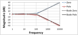
  Figure 2: Bode magnitude plot for zero and low-laissez passer pole; curves labeled "Bode" are the straight-line Bode plots

• 

  Effigy 3: Bode phase plot for zero and low-pass pole; curves labeled "Bode" are the directly-line Bode plots

• 

  Figure 4: Bode magnitude plot for pole-nil combination; the location of the zero is ten times college than in Figures two and three; curves labeled "Bode" are the straight-line Bode plots

• 

  Effigy five: Bode stage plot for pole-zippo combination; the location of the zero is x times college than in Figures 2 and iii; curves labeled "Bode" are the straight-line Bode plots

Gain margin and stage margin [edit]

Bode plots are used to assess the stability of negative feedback amplifiers by finding the proceeds and phase margins of an amplifier. The notion of proceeds and phase margin is based upon the gain expression for a negative feedback amplifier given by

${\displaystyle A_{\mathrm {FB} }={\frac {A_{\mathrm {OL} }}{i+\beta A_{\mathrm {OL} }}}\;,}$

where A_FB is the gain of the amplifier with feedback (the closed-loop gain), β is the feedback factor and A _OL is the gain without feedback (the open-loop gain). The gain A _OL is a complex function of frequency, with both magnitude and phase.^{[note one]} Test of this relation shows the possibility of infinite proceeds (interpreted equally instability) if the production βA _OL = −1. (That is, the magnitude of βA _OL is unity and its stage is −180°, the so-called Barkhausen stability criterion). Bode plots are used to determine just how close an amplifier comes to satisfying this status.

Central to this determination are two frequencies. The kickoff, labeled here equally f ₁₈₀, is the frequency where the open up-loop gain flips sign. The second, labeled here f _0 dB, is the frequency where the magnitude of the product | β A _OL | = i (in dB, magnitude 1 is 0 dB). That is, frequency f ₁₈₀ is determined by the condition:

${\displaystyle \beta A_{\mathrm {OL} }\left(f_{180}\right)=-|\beta A_{\mathrm {OL} }\left(f_{180}\right)|=-|\beta A_{\mathrm {OL} }|_{180}\;,}$

where vertical bars denote the magnitude of a complex number (for case, ${\displaystyle |a+\mathrm {j} b|=\left[a^{2}+b^{2}\correct]^{\frac {1}{two}}}$ ), and frequency f _0 dB is determined by the condition:

${\displaystyle |\beta A_{\mathrm {OL} }\left(f_{\mathrm {0dB} }\right)|=1\;.}$

1 measure of proximity to instability is the gain margin. The Bode phase plot locates the frequency where the phase of βA _OL reaches −180°, denoted here as frequency f ₁₈₀. Using this frequency, the Bode magnitude plot finds the magnitude of βA _OL. If |βA _OL|₁₈₀ ≥ ane, the amplifier is unstable, equally mentioned. If |βA _OL|₁₈₀ < 1, instability does not occur, and the separation in dB of the magnitude of |βA _OL|₁₈₀ from |βA _OL| = 1 is called the gain margin. Considering a magnitude of one is 0 dB, the gain margin is simply i of the equivalent forms: ${\displaystyle twenty\log _{x}(|\beta A_{\mathrm {OL} }|_{180})=20\log _{10}(|A_{\mathrm {OL} }|)-20\log _{10}(\beta ^{-i})}$ .

Another equivalent measure of proximity to instability is the phase margin. The Bode magnitude plot locates the frequency where the magnitude of |βA _OL| reaches unity, denoted here as frequency f _0 dB. Using this frequency, the Bode stage plot finds the phase of βA _OL. If the phase of βA _OL( f _0 dB) > −180°, the instability status cannot be met at any frequency (considering its magnitude is going to be < 1 when f = f ₁₈₀), and the distance of the phase at f _0 dB in degrees in a higher place −180° is chosen the phase margin.

If a simple yeah or no on the stability issue is all that is needed, the amplifier is stable if f _0 dB < f ₁₈₀. This criterion is sufficient to predict stability only for amplifiers satisfying some restrictions on their pole and nix positions (minimum phase systems). Although these restrictions usually are met, if they are not another method must be used, such as the Nyquist plot.^{[6] [seven]} Optimal gain and phase margins may be computed using Nevanlinna–Pick interpolation theory.^[eight]

Examples using Bode plots [edit]

Figures 6 and seven illustrate the gain behavior and terminology. For a iii-pole amplifier, Figure 6 compares the Bode plot for the gain without feedback (the open-loop gain) A _OL with the gain with feedback A _FB (the closed-loop gain). Run into negative feedback amplifier for more detail.

In this example, A _OL = 100 dB at low frequencies, and 1 / β = 58 dB. At depression frequencies, A _FB ≈ 58 dB too.

Because the open-loop gain A _OL is plotted and non the product β A _OL, the condition A _OL = one / β decides f _0 dB. The feedback gain at depression frequencies and for big A _OL is A _FB ≈ ane / β (wait at the formula for the feedback proceeds at the first of this section for the example of large proceeds A _OL), so an equivalent style to find f _0 dB is to expect where the feedback proceeds intersects the open up-loop gain. (Frequency f _0 dB is needed afterward to find the stage margin.)

Near this crossover of the two gains at f _0 dB, the Barkhausen criteria are well-nigh satisfied in this example, and the feedback amplifier exhibits a massive meridian in proceeds (it would be infinity if β A _OL = −i). Beyond the unity gain frequency f _0 dB, the open-loop gain is sufficiently small-scale that A _FB ≈ A _OL (examine the formula at the beginning of this section for the case of small A _OL).

Figure 7 shows the corresponding phase comparing: the phase of the feedback amplifier is nearly zilch out to the frequency f ₁₈₀ where the open-loop proceeds has a phase of −180°. In this vicinity, the phase of the feedback amplifier plunges abruptly downward to become almost the same as the phase of the open up-loop amplifier. (Recall, A _FB ≈ A _OL for pocket-sized A _OL.)

Comparison the labeled points in Figure half dozen and Figure 7, it is seen that the unity gain frequency f _0 dB and the phase-flip frequency f ₁₈₀ are very nearly equal in this amplifier, f ₁₈₀ ≈ f _0 dB ≈ 3.332 kHz, which means the proceeds margin and phase margin are nearly aught. The amplifier is borderline stable.

Figures eight and nine illustrate the gain margin and phase margin for a dissimilar amount of feedback β. The feedback gene is chosen smaller than in Figure 6 or 7, moving the condition | β A _OL | = 1 to lower frequency. In this example, 1 / β = 77 dB, and at low frequencies A _FB ≈ 77 dB as well.

Figure 8 shows the gain plot. From Figure 8, the intersection of 1 / β and A _OL occurs at f _0 dB = 1 kHz. Notice that the acme in the gain A _FB nigh f _0 dB is almost gone.^{[note 2] [9]}

Effigy 9 is the phase plot. Using the value of f _0 dB = 1 kHz found above from the magnitude plot of Effigy eight, the open-loop phase at f _0 dB is −135°, which is a phase margin of 45° higher up −180°.

Using Effigy ix, for a phase of −180° the value of f ₁₈₀ = 3.332 kHz (the aforementioned result as establish earlier, of class^{[note 3]}). The open-loop proceeds from Figure 8 at f ₁₈₀ is 58 dB, and 1 / β = 77 dB, so the proceeds margin is 19 dB.

Stability is not the sole criterion for amplifier response, and in many applications a more stringent demand than stability is good step response. As a rule of thumb, good step response requires a phase margin of at least 45°, and ofttimes a margin of over 70° is advocated, particularly where component variation due to manufacturing tolerances is an consequence.^[ix] See also the give-and-take of stage margin in the step response article.

• Examples

• 

  Effigy 6: Gain of feedback amplifier A _FB in dB and corresponding open-loop amplifier A _OL. Parameter ane/β = 58 dB, and at low frequencies A _FB ≈ 58 dB as well. The gain margin in this amplifier is nearly zero because | βA _OL| = 1 occurs at almost f = f _180°.

• 

  Effigy 7: Phase of feedback amplifier °A _FB in degrees and respective open-loop amplifier °A _OL. The phase margin in this amplifier is nearly goose egg because the phase-flip occurs at almost the unity gain frequency f = f _0 dB where | βA _OL| = 1.

• 

  Figure 8: Proceeds of feedback amplifier A _FB in dB and respective open-loop amplifier A _OL. In this example, 1 / β = 77 dB. The gain margin in this amplifier is 19 dB.

• 

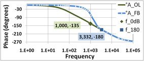
  Figure ix: Phase of feedback amplifier A _FB in degrees and respective open-loop amplifier A _OL. The phase margin in this amplifier is 45°.

Bode plotter [edit]

Effigy 10: Amplitude diagram of a tenth gild electronic filter plotted using a Bode Plotter awarding.

The Bode plotter is an electronic instrument resembling an oscilloscope, which produces a Bode diagram, or a graph, of a circuit's voltage gain or stage shift plotted confronting frequency in a feedback command organization or a filter. An example of this is shown in Figure 10. It is extremely useful for analyzing and testing filters and the stability of feedback control systems, through the measurement of corner (cutoff) frequencies and gain and phase margins.

This is identical to the function performed by a vector network analyzer, but the network analyzer is typically used at much higher frequencies.

For educational activity/enquiry purposes, plotting Bode diagrams for given transfer functions facilitates better understanding and getting faster results (encounter external links).

[edit]

Two related plots that display the same data in different coordinate systems are the Nyquist plot and the Nichols plot. These are parametric plots, with frequency as the input and magnitude and phase of the frequency response as the output. The Nyquist plot displays these in polar coordinates, with magnitude mapping to radius and stage to argument (bending). The Nichols plot displays these in rectangular coordinates, on the log scale.

• 

  Figure 12: A Nichols plot of the same response from Figure xi.

Meet also [edit]

• Analog signal processing
• Phase margin
• Bode's sensitivity integral
• Bode's magnitude (gain)–phase relation
• Electrochemical impedance spectroscopy

Notes [edit]

1. ^ Commonly, as frequency increases the magnitude of the gain drops and the phase becomes more than negative, although these are only trends and may be reversed in particular frequency ranges. Unusual gain behavior can render the concepts of gain and stage margin inapplicable. So other methods such every bit the Nyquist plot have to be used to appraise stability.
2. ^ The critical amount of feedback where the top in the gain merely disappears birthday is the maximally flat or Butterworth design.
3. ^ The frequency where the open-loop proceeds flips sign f ₁₈₀ does not modify with a change in feedback factor; it is a property of the open-loop gain. The value of the gain at f ₁₈₀ also does not change with a alter in β. Therefore, we could use the previous values from Figures vi and seven. Withal, for clarity the procedure is described using only Figures eight and 9.

References [edit]

1. ^ R. K. Rao Yarlagadda (2010). Analog and Digital Signals and Systems . Springer Scientific discipline & Business Media. p. 243. ISBN978-1-4419-0034-0.
2. ^ Van Valkenburg, M. E. University of Illinois at Urbana-Champaign, "In memoriam: Hendrik W. Bode (1905-1982)", IEEE Transactions on Automatic Control, Vol. AC-29, No iii., March 1984, pp. 193-194. Quote: "Something should be said about his proper name. To his colleagues at Bell Laboratories and the generations of engineers that have followed, the pronunciation is boh-dee. The Bode family unit preferred that the original Dutch exist used as boh-dah."
3. ^ "Vertaling van postbode, NL>EN". mijnwoordenboek.nl. Retrieved 2013-ten-07 .
4. ^ David A. Mindell Between Human and Machine: Feedback, Control, and Computing Earlier Cybernetics JHU Press, 2004 ISBN 0801880572, pp. 127-131
5. ^ Skogestad, Sigurd; Postlewaite, Ian (2005). Multivariable Feedback Control. Chichester, Due west Sussex, England: John Wiley & Sons, Ltd. ISBN0-470-01167-X.
6. ^ Thomas H. Lee (2004). The pattern of CMOS radio-frequency integrated circuits (Second ed.). Cambridge Great britain: Cambridge University Printing. p. §14.six pp. 451–453. ISBN0-521-83539-9.
7. ^ William S Levine (1996). The control handbook: the electrical engineering science handbook series (Second ed.). Boca Raton FL: CRC Press/IEEE Printing. p. §x.1 p. 163. ISBN0-8493-8570-9.
8. ^ Allen Tannenbaum (February 1981). Invariance and Systems Theory: Algebraic and Geometric Aspects. New York, NY: Springer-Verlag. ISBN9783540105657.
9. ^ ^{a b} Willy M C Sansen (2006). Analog design essentials. Dordrecht, The netherlands: Springer. pp. 157–163. ISBN0-387-25746-2.

External links [edit]

Wikimedia Eatables has media related to Bode plots.

• How to depict piecewise asymptotic Bode plots
• Gnuplot lawmaking for generating Bode plot: DIN-A4 printing template (pdf)

Source: https://en.wikipedia.org/wiki/Bode_plot

Posted by: kussreearly.blogspot.com

Share this post